When it comes to SETI, Radwave Explorer is where the fun happens. Here you can interactively explorer data collections that were processed by Radwave Engine.

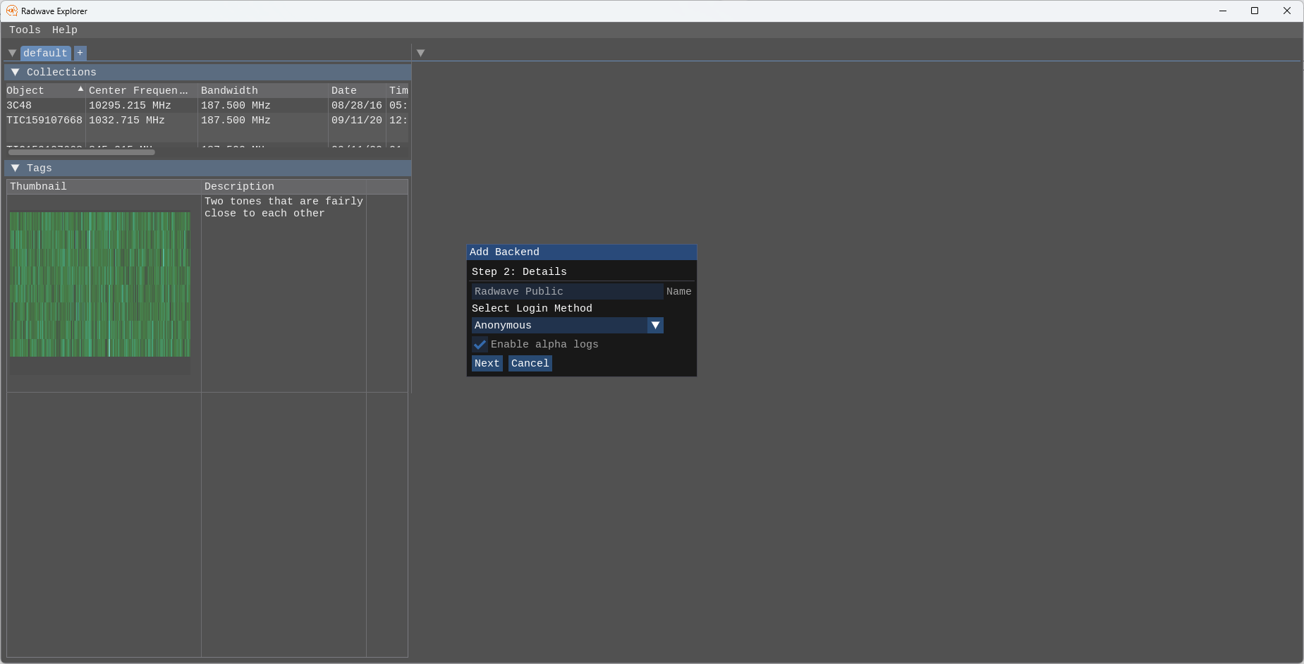
Alpha versions of Radwave will prompt you to log in on startup

Once logged in, you'll notice that the Radwave Public backend is now available. The collection within that backend is currently too dated to work, so please ignore it, and click the "default" tab at the top of the left sidebar. The sidebar can be resized to view all the columns

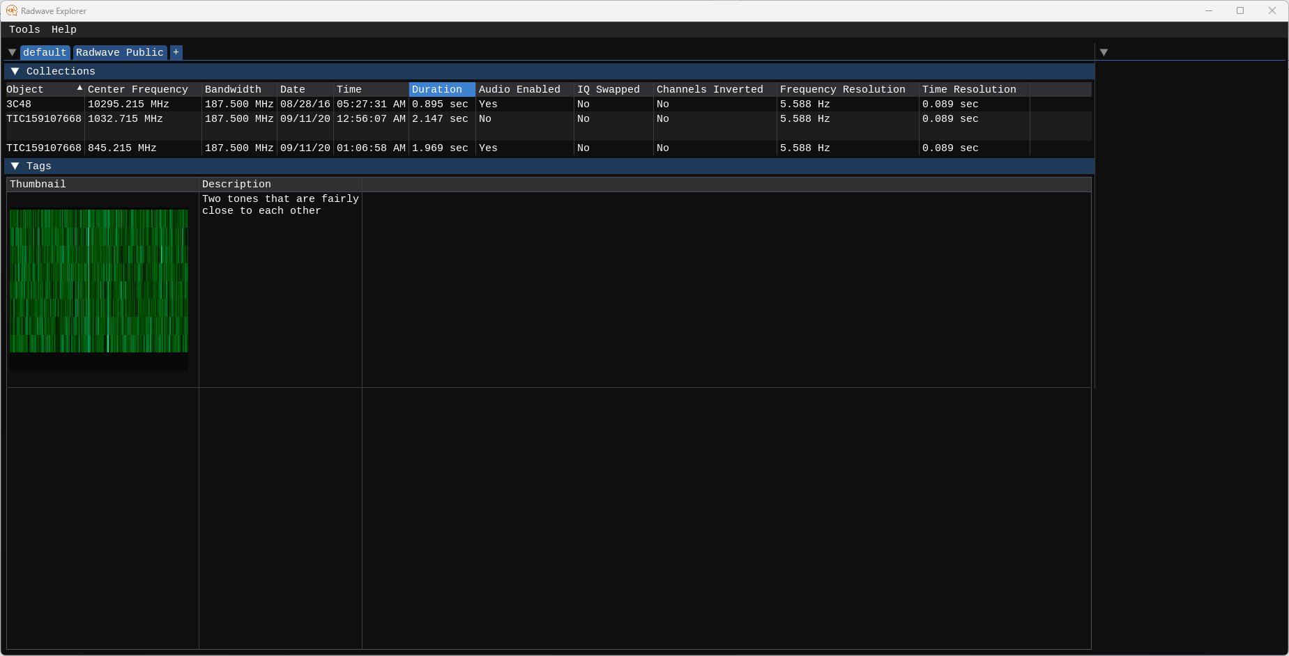
Here we can see the 3C48 collection from the Radwave Engine Tutorial. From what I can tell, there aren't as many clearly visible signals in 3C48 vs TIC159107668, so we'll look at that collection for now.

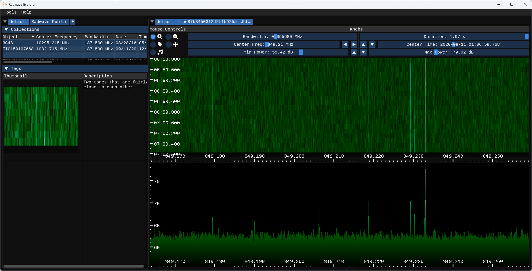
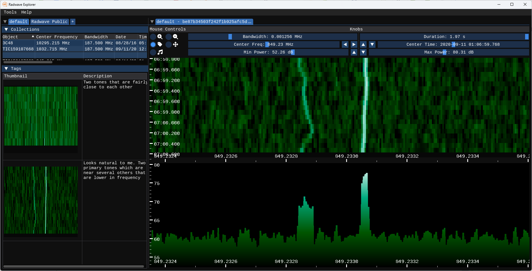
Upon opening it, we see two plots. The top is a spectrogram, with frequency on the horizontal axis and time on the vertical axis. The bottom is a power spectral density plot (PSD), with frequency on the horizontal axis and power on the vertical axis

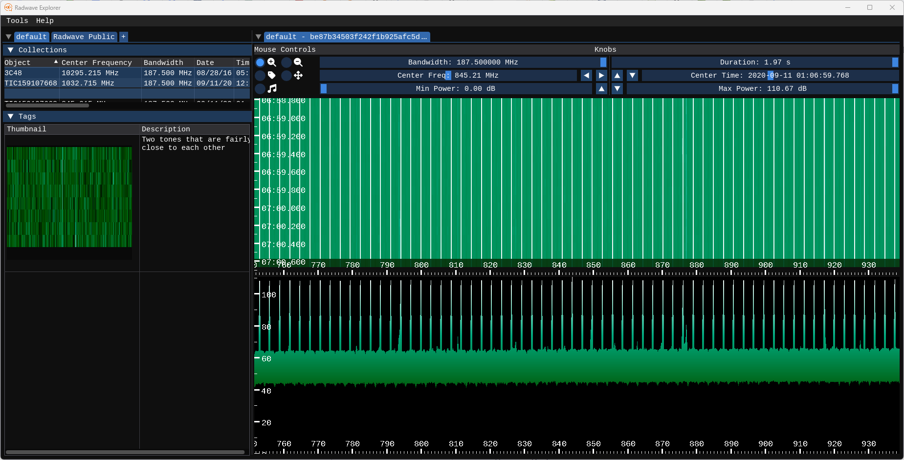
The first thing that stands out at the vertical white lines in the spectrogram and corresponding peaks in the PSD. We can use the mouse or the knobs at the tops to zoom into of those to better understand what we're looking at:

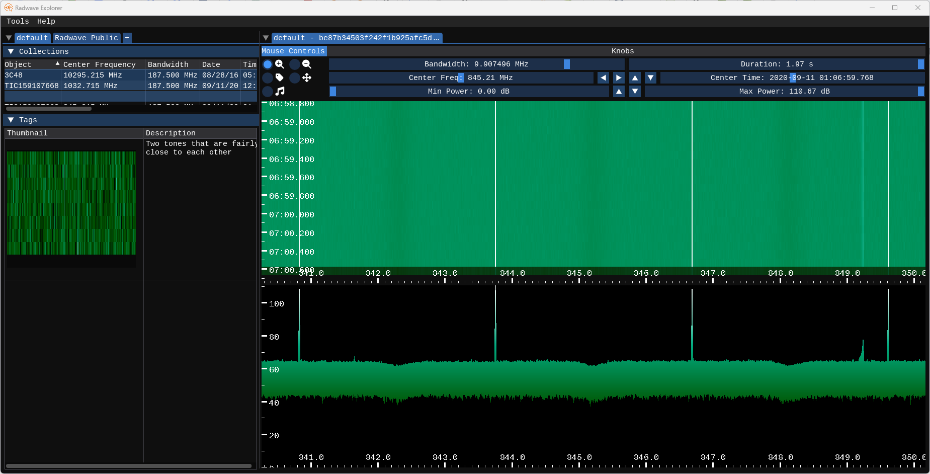
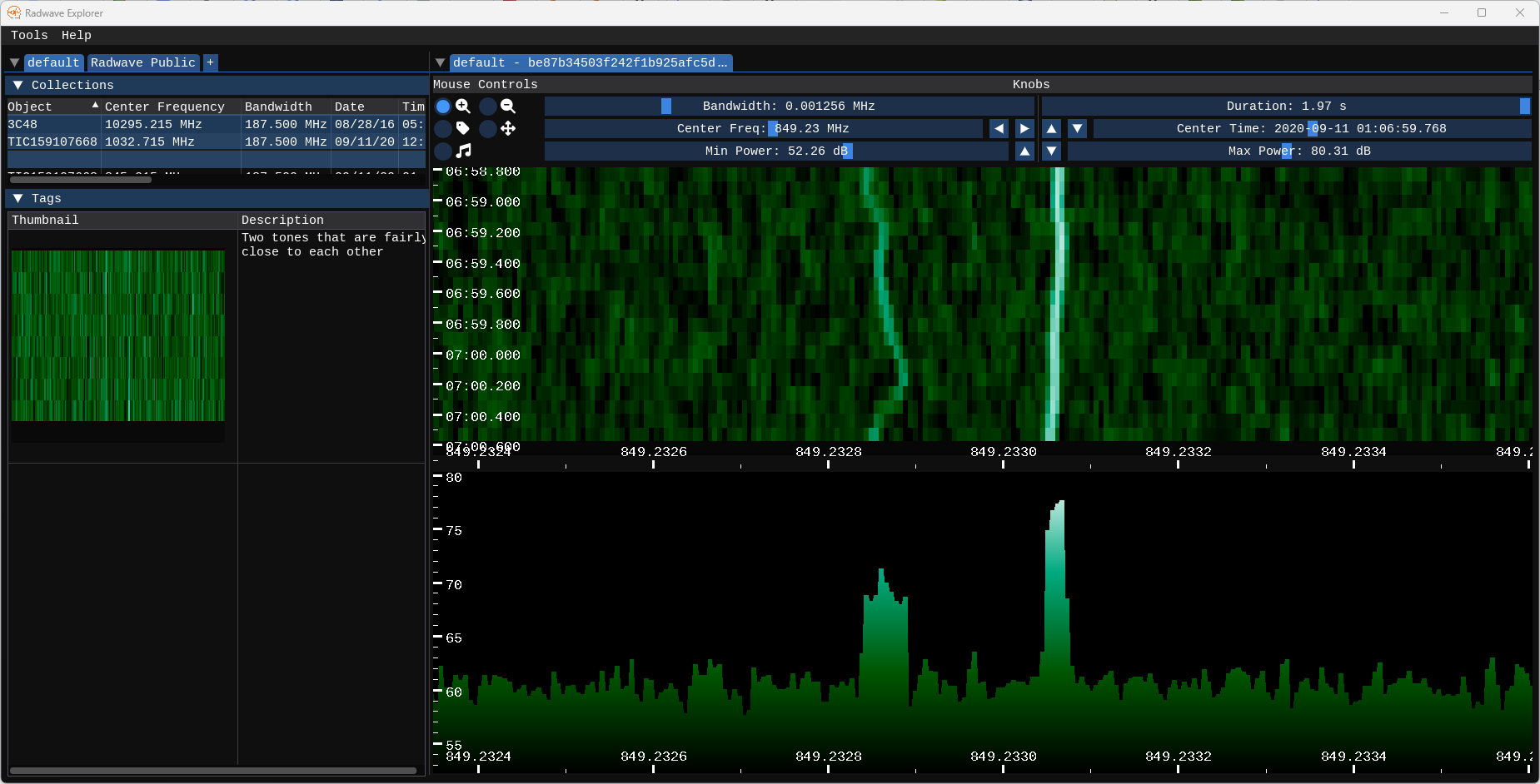
The receiver on the Green Bank Telescope (GBT) is channelized into 64 channels. At the center of each channel is a spike, which is likely due to either the local receiver's oscillator, or potentially standing voltage on the antenna. In either case, those main peaks are artifacts of the receiver, not actual signals. Additionally, you can see dips in the PSD midway between the peaks. This is due to the filters applied in the receiver chain. But on the right side, we can see a peak that's not due to the receiver. We can zoom in on it further, both in frequency and in power so that we make it easier to see the signal content.

And we can zoom in further on an individual peak

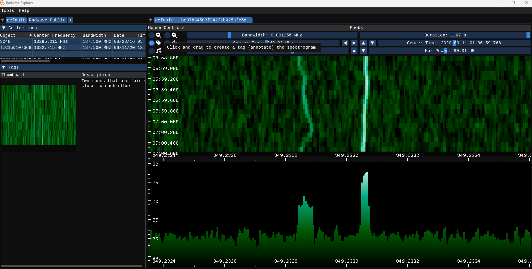
At this level we can really start to see the dynamic nature of the signals. Since we've found something cool, we can use the "tag" tool to save it

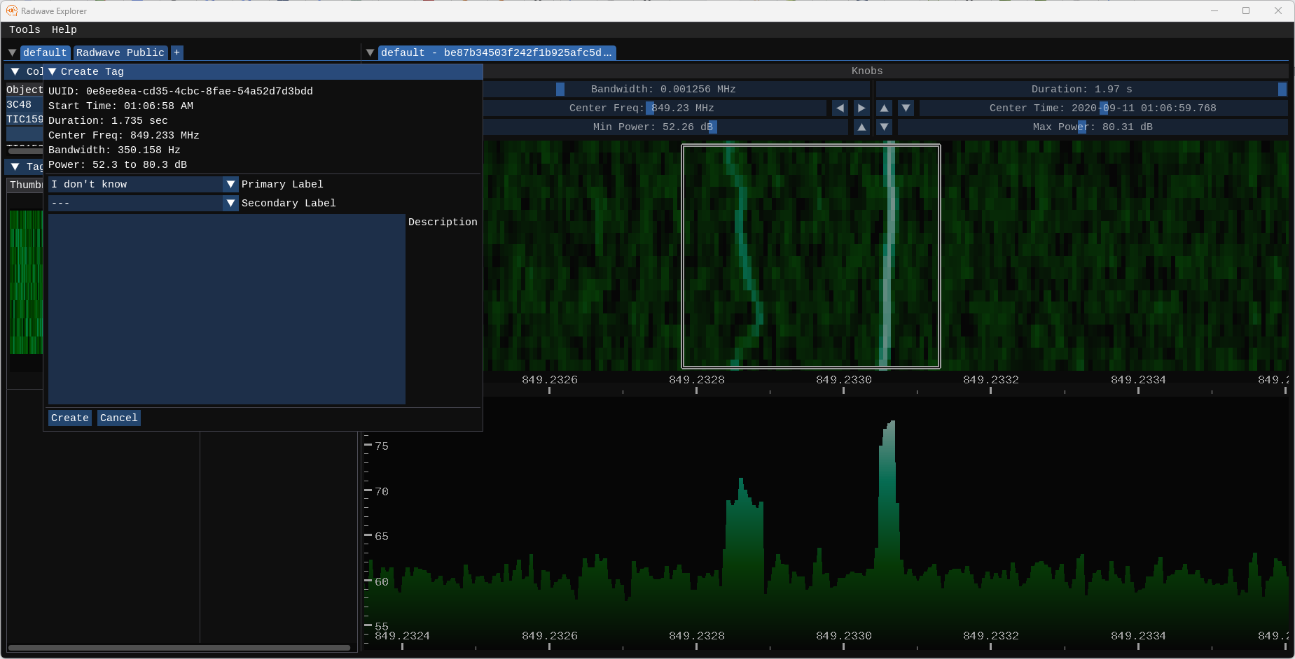
Once you create the tag, it'll appear in the tag list so that you can easily go back to it later.

Since we enabled audio for this collection, we can also extract audio

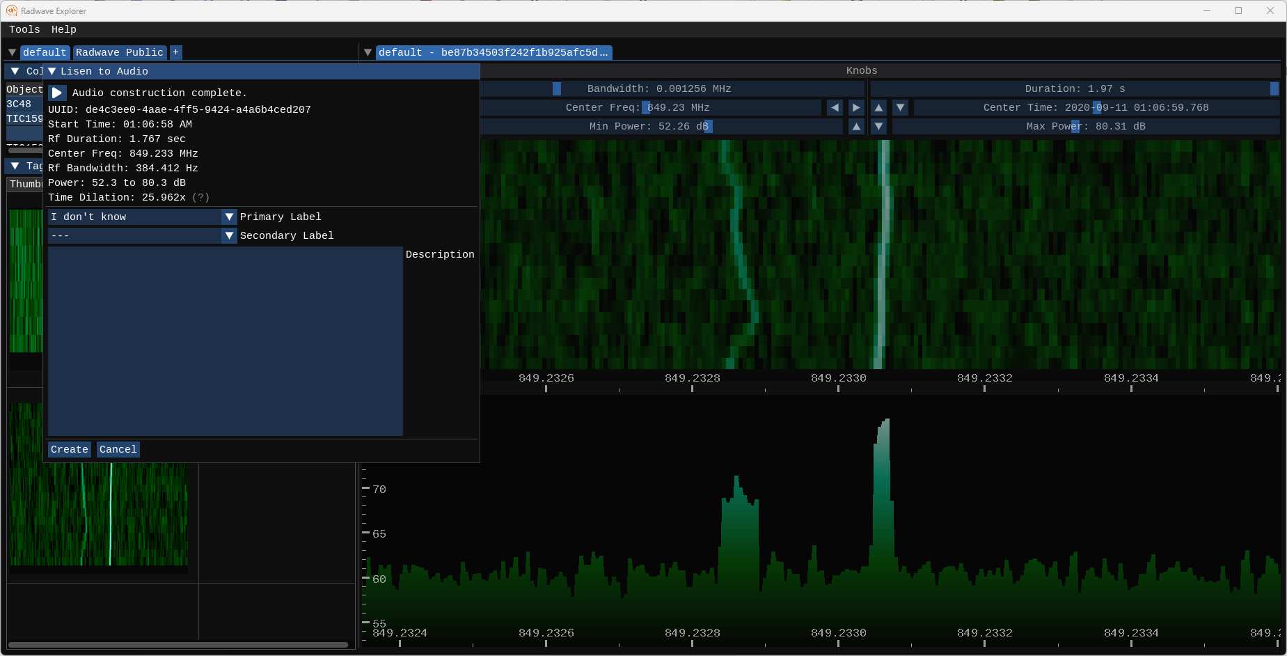
In this case, the time dilation is almost 26x for a 1.767 second capture, so the audio will be too short to meaningfully hear. We'll need to process a longer collection to get better audio, but we at least know which object and which frequencies to look for.

Radwave Explorer include configuration options much like the Engine. One key aspect though is our ability to connect to HTTP Backends in addition to Local Backends. This enables Radwave users to view collections that other users have processed. It should be noted that at this point, Radwave would benefit GREATLY from some people networking expertise who could help with the network security aspects of this, so I currently recommend only connecting to HTTP backends hosted on machines that you trust. If you know of someone who could help with network security, please reach out to me on the Radwave Discord channel! Thanks in advance!

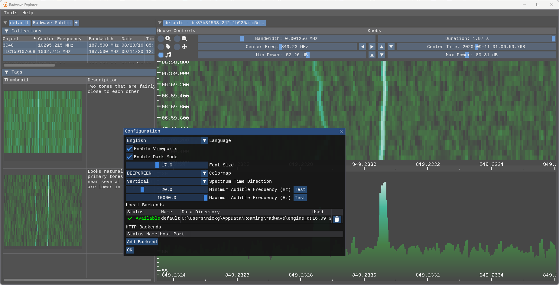
For audio, we can set the minimum and maximum audible frequencies. I personally don't enjoy listening to tones much above 5 kHz, but your preferences may be different. When you draw a box to extract audio, the leftmost frequency of the box is mapped to the minimum audible frequency, and the rightmost is mapped to the maximum audible frequency. So you can imagine the box you draw like a piano, with the low notes on the left and high notes on the right. Depending on where you draw the box, the signal will sound different.

That's a wrap for now! Happy listening!